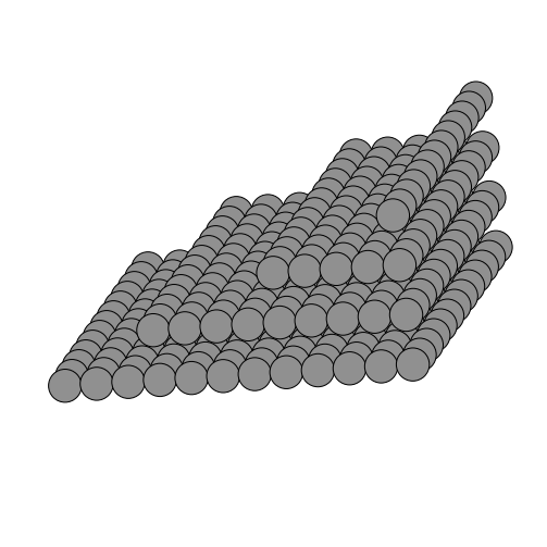
Quantification
Atomap contains two methods for performing quantification of atomic-resolution electron microscopy images.
The methods termed “Absolute Integrator” integrate over Voronoi cells or watershedded regions and compare the intensity in this region to the total beam intensity. When normalising for the detector response an accurate estimate of the percentage of the beam incident on the ADF detector for each atomic column can be obtained, which can be related to the scattering cross-section.
Atomap also contains an implementation of the “Statistical” method of ADF atomic-resolution quantification. In this method, the intensity of a Gaussian fit to each atomic column is plotted as a histogram. A Gaussian mixture model is then fit to this distribution, with each Gaussian corresponding to a different number of atoms in the columns.
Absolute Integrator
The absolute integrator function expects signals in the form of HyperSpy Signal2Ds where the Signal dimension looks like an atomic lattice. The Voronoi integrator function can take additional dimensions (such as EDS, EELS or 4D-STEM) as navigation dimensions. The Watershed integrator can only take 2D-datasets.
As an example using the nanoparticle dataset from the Atomap-demos repository, we can integrate over the atomic columns, letting the Voronoi cells expand infinitely.
>>> import atomap.api as am
>>> s = am.dummy_data.get_nanoparticle_signal()
>>> points_x, points_y = am.get_atom_positions(s, separation=4).T
>>> integrated_intensity, intensity_record, point_record = am.integrate(s, points_x, points_y)
>>> intensity_record.plot(cmap='viridis')
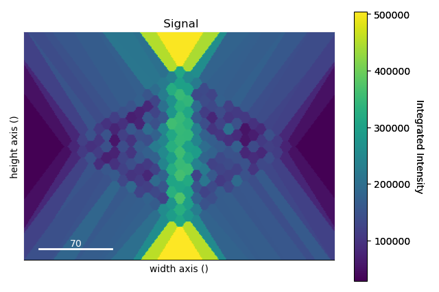
The infinitely expanding cells make it difficult for the eye to interpret the image. There are two ways to handle this:
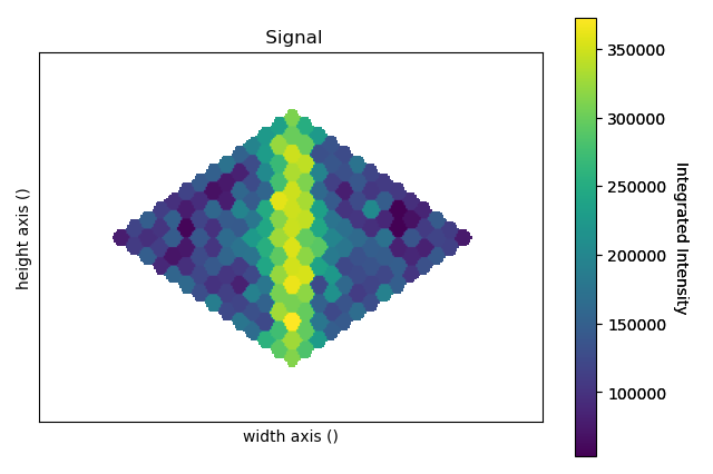
One can remove any cells that exist a certain distance from the image border, effectively removing one layer of atoms around the nanoparticle. This functionality is also optionally callable from the integrate function with remove_edge_cells=True.
>>> from atomap.tools import remove_integrated_edge_cells
>>> integrated_intensity, intensity_record, point_record = remove_integrated_edge_cells(integrated_intensity, intensity_record, point_record, edge_pixels=30)
>>> intensity_record.plot(cmap='viridis')
Alternatively one can specify the max_radius argument in order to limit the growth of the Voronoi cells:
>>> integrated_intensity, intensity_record, point_record = am.integrate(s, points_x, points_y, max_radius=5)
>>> intensity_record.plot(cmap='viridis')
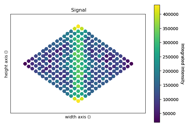
The integrated_intensity object contains a numpy array of intensities. The intensities refer to the atomic columns by their array index, and the indices can be visualised in the points_record object.
The following section describes methods incorporated from the AbsoluteIntegrator code for normalisation and quantification of ADF STEM images.
Detector Normalisation
detector_normalisation()
To carry out normal detector normalisation only the detector image and experimental image are needed.
>>> import hyperspy.api as hs
>>> import atomap.api as am
>>> det_image = am.example_data.get_detector_image_signal()
>>> image = am.dummy_data.get_simple_cubic_signal(image_noise=True)
>>> image_normalised = am.quant.detector_normalisation(image, det_image, 60)
Flux Weighting Analysis
In order to have a flux exponent to include in the detector normalisation (above), a flux analysis must be carried out. The detector flux weighting method is based on the paper G.T. Martinez et al. Ultramicroscopy 2015, 159.
>>> image_normalised = am.quant.detector_normalisation(image, det_image, inner_angle=60, outer_angle = None, flux_expo=2.873)
If the flux_exponent is unknown then it is possible to create an interactive flux plot described in detail in the example notebook: https://github.com/atomap-dev/atomap-demos/blob/release/adf_quantification_notebook/adf_quantification.ipynb
Statistical Method
For more information about the method itself, see S. Van Aert et al, Phys. Rev. B 87 (2013).
In order to perform the “statistical method” you must first have a Sublattice defined and you must also have used the Gaussian refinement.
>>> import atomap.api as am
>>> s = am.dummy_data.get_atom_counting_signal()
>>> atom_positions = am.get_atom_positions(s, 8, threshold_rel=0.1)
>>> sublattice = am.Sublattice(atom_positions, s)
>>> sublattice.construct_zone_axes()
>>> sublattice.refine_atom_positions_using_2d_gaussian()
Get number of Gaussians in GMM
Unless you already know the number of Gaussians to fit in your Gaussian mixture model, i.e. the number of different numbers of atoms in all of the columns, it is necessary to get this information. In order to obtain this number, you can fit Gaussian mixture models with different numbers of Gaussians and judge the best model by an information criterion (here we plot both AIC and BIC). Typically, a large negative gradient in the AIC/BIC is associated with the correct number of Gaussians, i.e. you’re looking for a local minimum.
To obtain plots of AIC and BIC for your image, you use the get_statistical_quant_criteria() function.
>>> models = am.quant.get_statistical_quant_criteria([sublattice], 10)
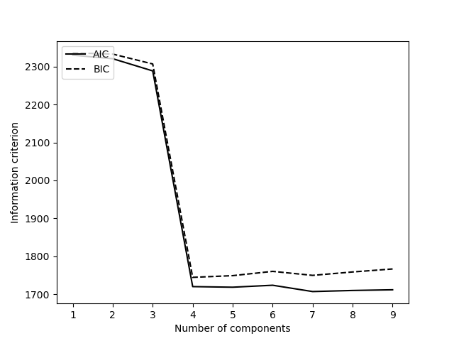
The get_statistical_quant_criteria() function takes a list of sublattices as an argument so that you can obtain a model for an individual image or a collection of images.
For multiple images make sure that they were all acquired with the same beam current and detector settings.
Apply the selected model
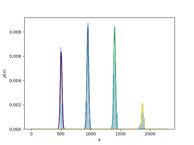
Once you have determined the number of Gaussians in your Gaussian mixture model, you can input this in to the statistical_quant() function.
>>> model = models[3]  # 4th model
>>> z_spacing = 2.4  # Angstrom
>>> atom_lattice = am.quant.statistical_quant(sublattice, model, 4, 'C', z_spacing)
The function returns an Atom_Lattice object, in which each Sublattice corresponds to atomic columns of different atomic number.
If plotting is selected (as it is by default) this plots the histogram of column intensities with the Gaussian mixture model overlayed.
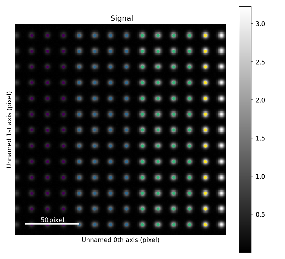
It also displays the image of the particle with sublattices coloured differently to indicate number of atoms in each column.
Finally, it will set the element_info attribute for each Atom_Position, which includes the element and z coordinates in Angstrom.
Visualise the selected model
The z_ordering parameter can be used to build the atomic columns in a given direction.
The z_ordering options are “bottom”, “top” and “center”. “center” can be useful for sperical nanoparticles.
For more info on working with atomic models with Atomap, see Working with Atomic Models.
>>> from ase.visualize import view
>>> sublattice.pixel_size = 0.1
>>> atom_lattice_1 = am.Atom_Lattice(sublattice_list=[sublattice])
>>> atoms = atom_lattice_1.convert_to_ase()
>>> view(atoms)
