Finding the atom lattice
The first step in using Atomap to analyse atomic resolution STEM images is to find the position of the atomic columns in the image. This tutorial will show how to do this from scratch:
Finding the feature separation
Generate initial positions for the atomic columns and initialize a
SublatticeobjectRefine the position of the atomic columns
Construct the zone axes
In this tutorial, the datasets from which the atomic positions are found are generated by using functionality in Atomap that generates test datasets. We will use an image of a simple cubic structure to introduce the basic steps.
After fitting a 2D-Gaussian to each atomic column a variety of structural information can be extracted: such as the distance between atoms and monolayers, and ellipticity. This will be dealt with in the Analysing atom lattices tutorial.
A simple cubic structure
The dataset used in this example will be generated using the atomap.dummy_data module:
>>> %matplotlib widget
>>> import atomap.api as am
>>> import numpy as np
>>> import atomap.dummy_data as dummy_data
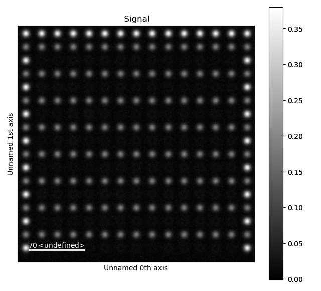
>>> s = dummy_data.get_simple_cubic_signal(image_noise=True)
>>> s.plot()
White noise was added to the image, in order to make it more realistic. To use your own images rather than this test dataset, load your own image for example by using HyperSpy. HyperSpy supports a large variety of image formats, for example dm3/dm4, tiff and emi/ser.
>>> import hyperspy.api as hs
>>> your_image = hs.load(your_filename)
We will continue with the test dataset s.
1. Finding the feature separation
Atomap finds initial positions for the atomic columns by using a peak finding algorithm from the python package skimage.
This algorithm needs to know the smallest peak separation (minimum pixel separation of the features).
You can find the optimal pixel separation by using the Atomap function get_feature_separation() which returns a HyperSpy signal.
>>> s_peaks = am.get_feature_separation(s, separation_range=(2, 20), show_progressbar=False)
This function uses the peak finding algorithm for a range of pixel separations.
The default separation range is 5 to 30.
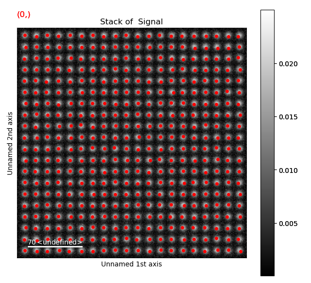
s_peaks is plotted below.
The left figure shows where the peak finding function has located a peak, the right figure shows the minimum feature separation in pixels on the x-axis.
Use the Ctrl key + left-right arrow keys to navigate through the different minimum feature separation, and see how it affects the result of the peak finding in the left figure.
>>> s_peaks.plot()
The requirements for the peak separation are:
With an optimal peak separation, only atoms from one sublattice should be marked.
In addition, all the atoms from the first sublattice should be marked. (It is not necessary that all the atoms at the edges are marked).
With a pixel separation of 2, too many atoms are found.

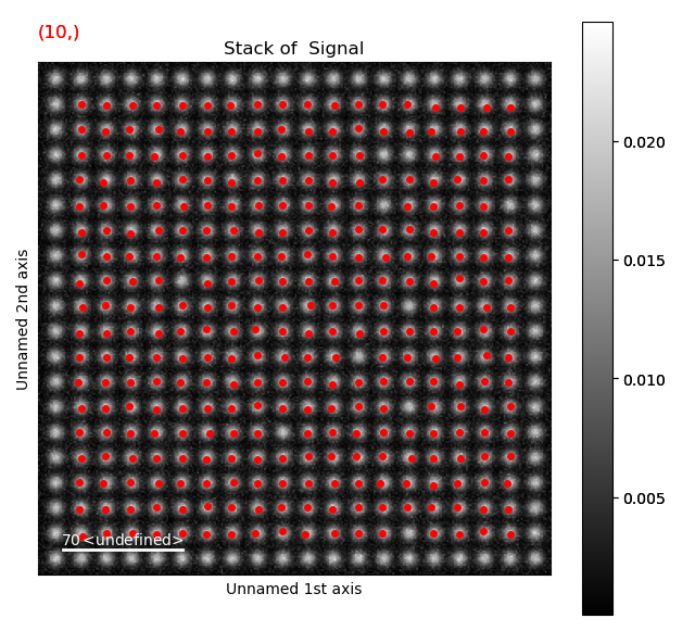
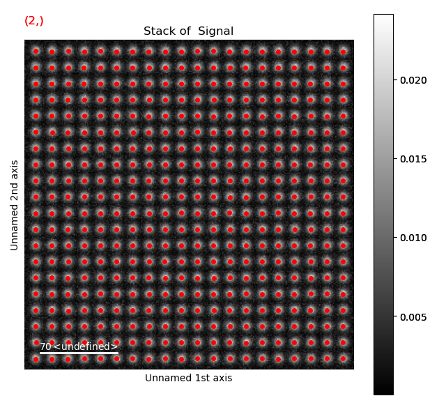
With a pixel separation of 7, all atoms are identified. Often, the program will have difficulties with finding the atoms in the rows at the boundary of the image. This does not matter, the important thing is that all atoms in the central part of the image are found.
12 is a too large pixel separation, as not all atoms in the interior of the image are found. This will create issues when the zone axes are constructed and atom planes are found (part 4).
2. Generate the initial positions for the atomic columns and initialize a Sublattice
Having found the optimal feature separation, it is time to generate the initial atomic positions.
get_atom_positions() takes the atomic resolution image signal s and the optimal feature separation.
The function also allows for PCA, relative threshold, background subtraction and normalization of intensity, these options are described in
the api documentation.
>>> atom_positions = am.get_atom_positions(s, separation=7)
atom_positions is a list of x and y coordinates of initial atom positions.
If there are any missing or extra atoms add_atoms_with_gui() can be used, see Adding atoms using GUI for more info.
If there are several phases within the image, these can be separated using select_atoms_with_gui(), see Several phases for more info.
This list will be used to initialize a Sublattice object, which will contain all the information about the atoms.
In our simple example, all atoms belong to the same sublattice, so only one Sublattice object is needed.
(In the more advanced example below, images containing more than one sublattice will be analysed).
The Sublattice object takes a list of atom positions, and a 2D NumPy array representing the image.
>>> sublattice = am.Sublattice(atom_positions, image=s.data)
>>> sublattice
<Sublattice,  (atoms:400,planes:0)>
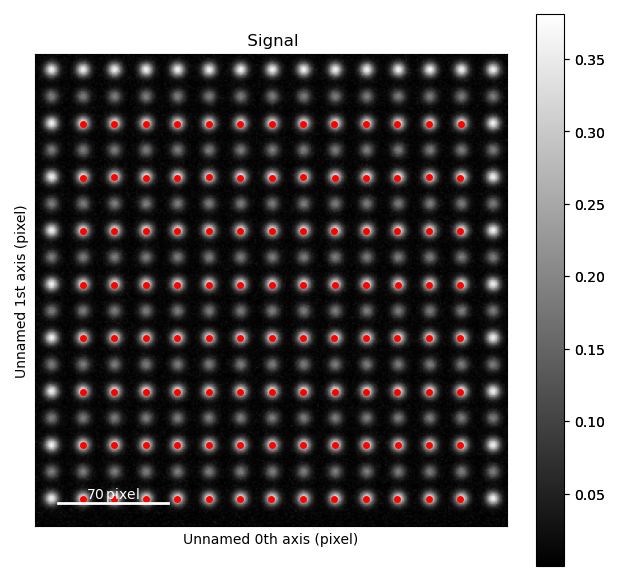
3. Refine the position of the atomic columns
Atomap uses centre of mass (refine_atom_positions_using_center_of_mass()) first,
and then 2D-Gaussians (refine_atom_positions_using_2d_gaussian()) to refine the positions (and shape) of the atomic columns.
Before the refinement, the nearest neighbours of each atomic column must be found.
This is needed to for Atomap to know boundary values for the position refinements, and is set using find_nearest_neighbors().
>>> sublattice.find_nearest_neighbors()
>>> sublattice.refine_atom_positions_using_center_of_mass()
>>> sublattice.refine_atom_positions_using_2d_gaussian()
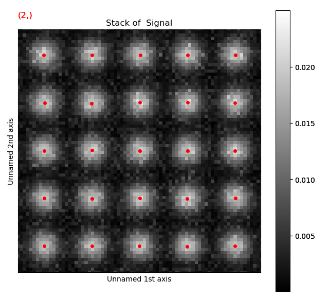
Let’s see what how the refinement procedure have improved the atom positions.
>>> sublattice.get_position_history().plot()
Again, navigate through from the initial positions, to the positions after the first and second refinement, in this case the centre of mass and 2D-Gaussian respectively. Below, the initial and end position are shown.
Atom positions have clearly been improved by the refinement. The quality of the fit is seen more clearly when we zoom in on the atoms.
Information on the atoms in a sublattice can always be accessed through sublattice.atom_list, which contains all the atom positions.
Each atom position is represented as the Atom_Position class.
>>> atom_list = sublattice.atom_list
>>> atom_list[0]
<Atom_Position,  (x:290.2,y:289.9,sx:3.1,sy:3.2,r:0.2,e:1.0)>
4. Construct zone axes
Atomap can find atom planes and zone axes in a Sublattice.
The program uses nearest neighbour statistics in real space, and finds the translation symmetry.
This is done using the construct_zone_axes() method.
If not all atoms in the interior of the image are found (as in the peak finding in part 2, with the largest feature separation), the atom planes will probably be discontinuous at the “missing atom”.
>>> sublattice.construct_zone_axes()
>>> sublattice
<Sublattice,  (atoms:400,planes:4)>
The zone axes are needed for the types of analysis explained in Analysing atom lattices.
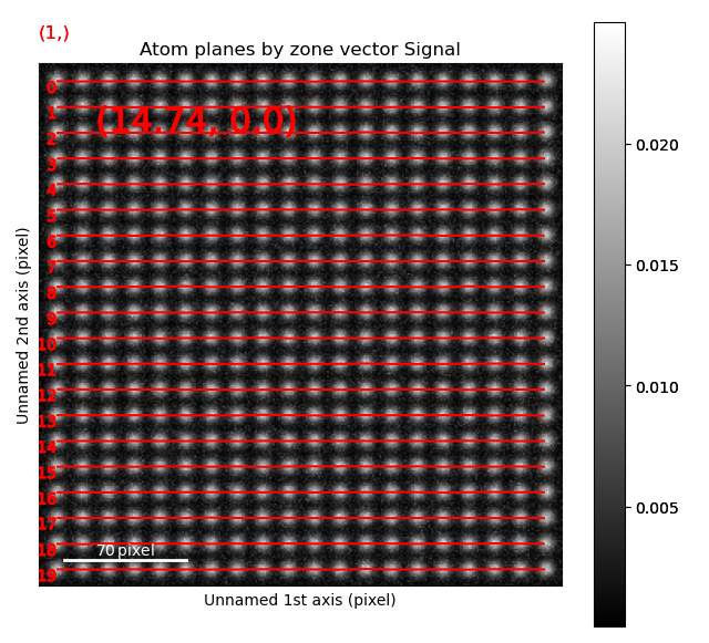
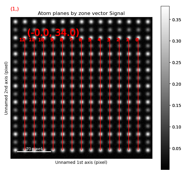
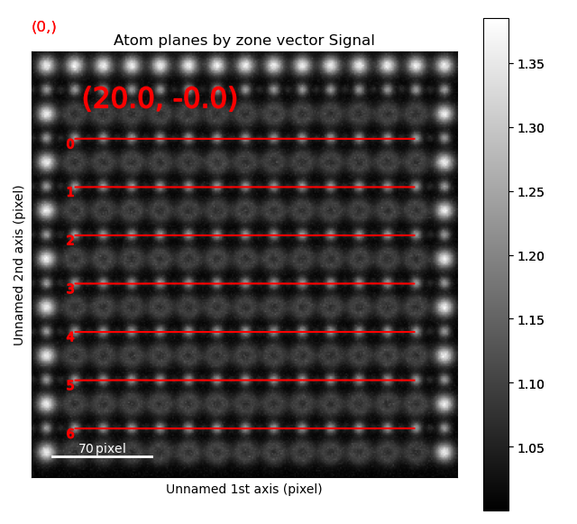
Atom planes for the zone axes in the sublattice can easily be plotted.
The atom planes are represented as Atom_Plane class objects,
which contains all the atoms in one plane, and the relation between these atoms.
>>> sublattice.plot_planes()
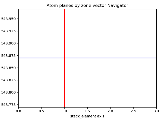
Navigate though the different zone vectors to see the corresponding planes (Ctrl + left-right arrow keys).
If you’re using your own dataset and some of the planes are non-continuous
or missing, try increasing the atom_plane_tolerance from the default 0.5:
sublattice.construct_zone_axes(atom_plane_tolerance=0.7).
If you want to get more atomic planes, increase the nearest_neighbor parameter from the default 15:
>>> sublattice_cubic = am.dummy_data.get_simple_cubic_sublattice()
>>> sublattice_cubic.construct_zone_axes(nearest_neighbors=25)
>>> sublattice_cubic
<Sublattice,  (atoms:400,planes:8)>
Images with more than one sublattice
Often, the STEM images will have more than one sublattice.
We will now find the atom positions in an image containing two sublattices, where the atomic columns in one of the sublattices are more intense than in the other.
Again, we use a dummy dataset generated using atomap.dummy_data.
First, the sublattice with the most intense columns is found.
The optimal feature separation is found the same way as the earlier example, and 15 was found to work well.
>>> s = dummy_data.get_two_sublattice_signal()
>>> A_positions = am.get_atom_positions(s, separation=15)
>>> sublattice_A = am.Sublattice(A_positions, image=s.data, color='r')
>>> sublattice_A.find_nearest_neighbors()
>>> sublattice_A.refine_atom_positions_using_center_of_mass()
>>> sublattice_A.refine_atom_positions_using_2d_gaussian()
>>> sublattice_A.construct_zone_axes()
>>> sublattice_A.plot()
>>> sublattice_A.plot_planes()
The atom positions are shown in the left image, and the atom planes for one zone axis is shown in the right.
This zone axis has index 1 in the list sublattice_A.zones_axis_average_distances.
Atomic columns belonging to the second, less intense sublattice (“B”) are between the “A” atoms in the most intense sublattice.
Knowing this, the trick to find the initial positions for the “B”-columns is using
find_missing_atoms_from_zone_vector():
>>> zone_axis_001 = sublattice_A.zones_axis_average_distances[1]
>>> B_positions = sublattice_A.find_missing_atoms_from_zone_vector(zone_axis_001)
In this case, the B-columns are exactly at the halfway point between the A-columns, however for other structures this
might not work.
If that is the case, use the vector_fraction parameter: sublattice_A.find_missing_atoms_from_zone_vector(zone_axis_001, vector_fraction=0.7).
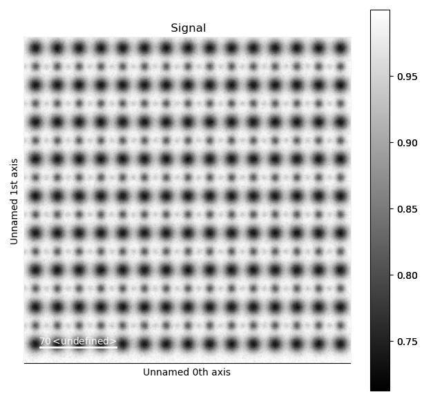
To enable robust fitting of the less intense B-positions, the intensity from the A-positions are “subtracted” from the image. This “subtracted”-image is then used to refine the B-positions.
>>> from atomap.tools import remove_atoms_from_image_using_2d_gaussian
>>> image_without_A = remove_atoms_from_image_using_2d_gaussian(sublattice_A.image, sublattice_A)
This is how the image looks like after the Gaussians fitted to the A-atoms are subtracted from the original image. Now, the B-positions can be refined without being drowned by the more intense A-positions.
>>> sublattice_B = am.Sublattice(B_positions, image_without_A, color='blue')
>>> sublattice_B.construct_zone_axes()
>>> sublattice_B.refine_atom_positions_using_center_of_mass()
>>> sublattice_B.refine_atom_positions_using_2d_gaussian()
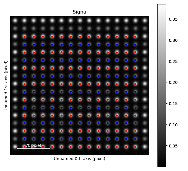
The sublattices can be contained within an Atom_Lattice object.
>>> atom_lattice = am.Atom_Lattice(image=s.data, name='test', sublattice_list=[sublattice_A, sublattice_B])
>>> atom_lattice.plot()
Sublattices can be accessed in Atom_Lattice.sublattice_list:
>>> sublattice_A = atom_lattice.sublattice_list[0]
The Atom_Lattice object with all the atom positions can be stored as a HDF5-file:
>>> atom_lattice.save("atom_lattice.hdf5", overwrite=True)
This will make a HDF5-file in the current working directory.
To restore the atom lattice, use the load_atom_lattice_from_hdf5() function:
>>> atom_lattice2 = am.load_atom_lattice_from_hdf5("atom_lattice.hdf5")
To save single sublattices, initialize an Atom_Lattice object with your sublattice as the only sublattice, and save the Atom_Lattice.
>>> import atomap.api as am
>>> sublattice = am.dummy_data.get_simple_cubic_sublattice()
>>> atom_lattice = am.Atom_Lattice(image=sublattice.image, sublattice_list=[sublattice])
>>> atom_lattice.save("simple_cubic_atom_lattice.hdf5", overwrite=True)
Finding the oxygen sublattice
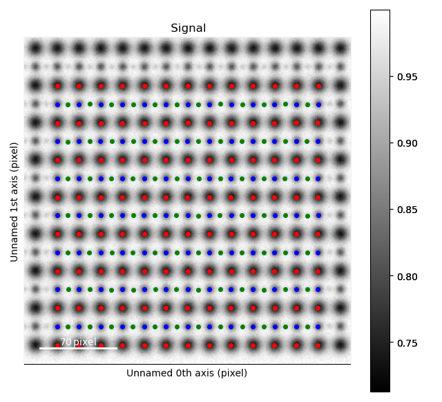
Light elements such as oxygen and fluorine can be imaged by using Annular Bright Field (ABF). While the sublattices of heavier atoms such as the A and B cations in perovskites are most easily imaged using Annular Dark Field (ADF) imaging, the ABF image can be used to find the oxygen positions. In this example, we will use the sublattices found above to find the third and last sublattice in an ABF type of image.
>>> s_ABF = am.dummy_data.get_perovskite110_ABF_signal(image_noise=True)
>>> s_ABF.plot()
First, we need to “subtract” the intensity of the A and B cations in this image. In practice this means that the A and B sublattices in the ABF image must be found. We already have good atom positions for both the A and B sublattice from above, and these positions will be used as initial positions. Furthermore, the inverse of the ABF image is used, such that the intensities of the atoms in the image are higher than the surroundings.
>>> initial_positions = sublattice_A.atom_positions
>>> sublattice_A2 = am.Sublattice(initial_positions, image=np.divide(1, s_ABF.data), color='r')
>>> sublattice_A2.find_nearest_neighbors()
>>> sublattice_A2.refine_atom_positions_using_center_of_mass()
>>> sublattice_A2.refine_atom_positions_using_2d_gaussian()
>>> sublattice_A2.construct_zone_axes()
>>> image_without_A2 = remove_atoms_from_image_using_2d_gaussian(sublattice_A2.image, sublattice_A2)
The same is done for the B-sublattice
>>> initial_positions = sublattice_B.atom_positions
>>> sublattice_B2 = am.Sublattice(initial_positions, image=image_without_A2, color='b')
>>> sublattice_B2.find_nearest_neighbors()
>>> sublattice_B2.refine_atom_positions_using_center_of_mass()
>>> sublattice_B2.refine_atom_positions_using_2d_gaussian()
>>> sublattice_B2.construct_zone_axes()
>>> sublattice_B2.plot_planes()
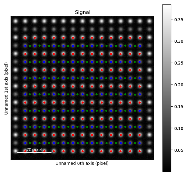
We know that the oxygen atoms are between B atoms in the horizontal direction. A similar method to the method for finding the first B-positions above, in the “ADF”-image, is used to find the O-columns in the “ABF” image.
>>> zone_axis_002 = sublattice_B2.zones_axis_average_distances[0]
>>> O_positions = sublattice_B2.find_missing_atoms_from_zone_vector(zone_axis_002)
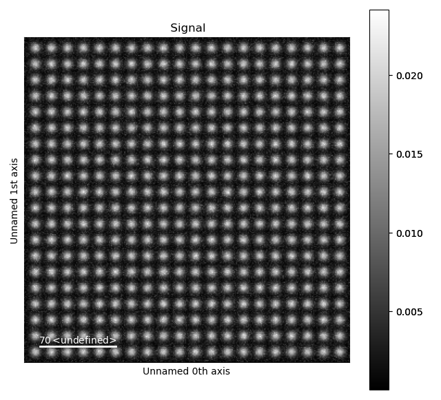
>>> image_without_AB = remove_atoms_from_image_using_2d_gaussian(sublattice_B2.image, sublattice_B2)
>>> sublattice_O = am.Sublattice(O_positions, image_without_AB, color='g')
>>> sublattice_O.construct_zone_axes()
>>> sublattice_O.refine_atom_positions_using_center_of_mass()
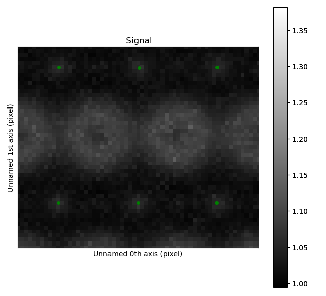
>>> sublattice_O.refine_atom_positions_using_2d_gaussian()
Zooming in to see some of the oxygen positions, indicated by the green dots.
All three sublattices can now be added to an atom lattice: The A and B sublattices from the ADF image, and the O-sublattice from the ABF image.
>>> atom_lattice = am.Atom_Lattice(image=s_ABF.data, name='ABO3', sublattice_list=[sublattice_A, sublattice_B, sublattice_O])
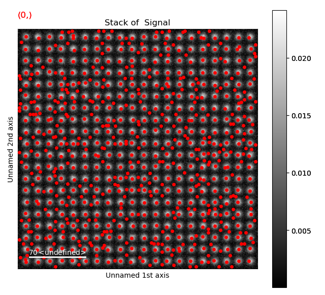
All sublattices can be visualized on the ADF and ABF image:
>>> atom_lattice.plot()
>>> atom_lattice.plot(image=s.data)